Welcome to our Wiki On this page, we want to give you some more information to better understand AI and especially the XAI methods, we use in our evaluation.
We believe real acceptance and a objective discussion can only come from a level playing field.
This requires knowledge about the systems, at least to a basic degree.

AI as well as XAI is no magic and works based on mathematical basics. But of course no system is perfect and we all need to know the potentials as well al the limits of AI.

When we refer to AI in this evaluation, most of the time our behind-the-scenes classification system is meant.
For our classification we used the AUCMEDI - Library to train a Convoluted Neural Network for image classification.
Lets break down what this means!
A neural network is depicted in the image to the side. This is a graphical representation of the mathematical system behind the classification. It works similar to a brain with nerves that have different activation potentials. An image is split into its pixel as the input (similar, to how our eyes have many little photon receptors for light), and the classification is the output (like our thoughts wenn we recognize for example a cat on an image).
Neural networks are great at learning complex tasks like shape recognition (,which is exactly what Gleason grading does).
Convoluted means it has convolutions in its layers, this is a technique, to better depict the local dependencies within images and their neighboring elements.
Classification means, the AI is classifying images.
We gave the AI images that were labelled "Gleason 3", "Gleason 4", "Regular" for example.
The task for the AI is, to correctly classify previously unseen images to the labels we gave before. In addition to this, the AI outputs a certainty score. It shows how certain it is, that each label is correct. This can be seen in the Bar-chart when hovering over a specific patch in the viewer.

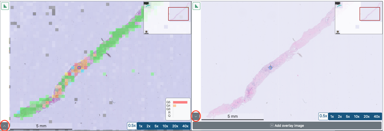
The "+ Add overlay image" button below the viewer fields allows you to overlay various eXplainable AI (XAI) visualizations on top of the samples.

Note, while the AI, based on Gleason grading, highlights pathologically abnormal tissue, the XAI colourizes areas that may be critical to the AI assessment. Here, possible similarities in color scheme between AI and XAI, do not necessarily indicate correlations. Each method and its color scheme must be considered independently of each other.

If you click on the button, a kind of table appears. On the far left, in the drop-down menu, under the title "Overlay" you can select the appropriate visualization.

• Gleason: An artificial intelligence which evaluates the sample based on the Gleason Score. Blue = questionable tissue ; Green = regular tissue ; Yellow = Gleason 3 ; Orange = Gleason 4 ; Red = Gleason 5
• sm: Saliency Map, an exposure map that increases the exposure of the pixel that causes the greatest change in the selection of the final Gleason Score class for that tile.
  In simple terms, it is a map that shows which pixels have a (positive or negative) impact on the decision.
  Unlike Grad-Cam, which analyses regions, Saliency Map focuses on individual pixels. Thus, the resulting XAI map consists of many small points.
• gc: Grad-Cam. - Gradient-weighted Class Activation Mapping (Grad-CAM).
  Highlighting of image regions by a gradient, a so-called heat map, which had a high gradient influence on the prediction or classification. Here the focus is on larger regions of an image that have a significant influence on the decision and therefore contain features or information that determine the classification results.
• gcpp: Grad-Cam++, similar to Grad-CAM, areas are also marked here, but this method uses a different gradient function of a higher order.
  Generally an extension of Grad-Cam that uses slightly different/extended formulas for calculating region effects. This method should therefore give similar results to Grad-CAM.
• gb: Guided Backpropagation, similar to saliency maps, this XAI also works at the pixel level but includes a "local smoothing factor". In simple terms, it uses edges or image features and tries to map the exposure/saliency map to the image features.
  In general, Guided Backpropagation looks a little "cleaner" because it highlights pixels on edges or features in the image, rather than the more "cloudy" pixel distribution of saliency maps. HOWEVER, the "local smoothing" results in potentially blurring important pixels just because they are not near an edge in the image.
  This can lead to misleading interpretations and highly distorted XAI maps, which is currently causing active discussion in the field.

The slider under the title "Opacity" allows you to adjust the intensity of the colorization, up or down, by dragging the slider to the right or left with the mouse held down. Using the options in the drop-down menu of the last column, titled "Colormap", you can change the color scheme of the visualization.
Finally, in the drop-down menu under the title "Composite Operations" you can choose between source over and color burn. These operations affect the way colors and textures of different elements and styles interact with each other.